Machine Visual Acuity

In this project, we aim to gain insights about human visual acuity by applying these tests to machines. The main goal is to first train a convolutional-based neural network to recognize optotypes with low amounts of distortions so that it can use its knowledge to classify an unseen optotype from a testing set with optotypes with medium to high amounts of distortions. We used transfer learning, with the use of a VGG network, to obtain a baseline model for the problem. Then, we experimented with mixing the testing set with the training set, to determine if that could help the network make better predictions.

Introduction

Motivation

In the field of Ophthalmology, the most commonly used methodology to test a patients’ visual sharpness, known here-throughout as “Visual Acuity”, is to perform a test such as depicted by the Snellen chart, shown in Figure 1. This method is so pervasive in the field that visual acuity tests are generally thought to be interchangeable with the testing of alphanumeric characters. However, it has been observed in the Browne Lab of Ophthalmology here at UC Irvine that the results of Visual Acuity tests do not yield consistent results for different character sets, known as “Optotypes.” Typically, these Optotypes do not even utilize the full range of characters in the alphabet, and instead are limited to about 5-10 different letters.

Figure 1: Snellen Chart, commonly used by Ophthalmologists to measure a patient's visual acuity, or ability to discern character sharpness.

Related Work

Other Visual Acuity tests outside of the standard use of alphanumeric characters have been developed to address specific needs for a small subset of patients. For instance, the Teller Acuity tests, depicted in Figure 2, use a series of parallel lines in varying width and gradients. This test was developed specifically for patients such as infants with low cognitive abilities who are not yet able to discern alphanumeric characters. However, as shown, even in images without any applied optical distortion, these are difficult to discern from each other. Patients who lack literacy, for example, do not necessarily possess low cognitive abilities, but would be at a disadvantage in participating in the Snellen-like acuity tests.

Figure 2: Teller acuity cards, used to measure visual acuity in patients with low cognitive abilities such as infants.

Project Overview and Goals

This project—conducted as a research project Brooke undertook in the Baldi Lab towards her Master’s thesis—is being jointly researched by the Browne Lab of Ophthalmology. Broadly, the goal is to explore what insights can be gained from applying a range of different acuity tests, as depicted in Figure 3, to both humans and machines. The machine tests are specifically conducted using Deep Neural Models, as this is the most accurate representation of human visual processing in the computer vision literature. For both the human and machine tests, it was necessary to digitally recreate the varying degrees of distortion that a patient would encounter in an Ophthalmologist’s office, which were graciously obtained from the Browne lab. The dataset is an aggregation of images of the optotypes with increasingly distorted images to increase the difficulty for the subject to discern the character.

Figure 3: Column 1 depicts the list of various Acuity libraries tested, with the corresponding row delineating the optotype characters that belong to it.

Experimentation

The primary Deep Learning technique that was applied to solve the problem, at least initially, was Transfer Learning. I primarily explored the use of VGG-16, while Andreana produced further successful results by using the deeper VGG-19 model and applying further fine-tuning of the model. This proved to be the most successful model that stays within the confines of the requirements of the original project. Andreana further explored if lifting some of those constraints resulted in higher accuracy, which ultimately it did.

Additionally, using techniques and concepts from this course, I applied data augmentation to the set of training images in order to bolster the range of both training and validation images available to the model. While this drastically improved validation accuracy of the low-distortion optotpyes, it resulted in lower accuracy for the high-distortion optotypes.

Evaluation and Results

This quarter, as well as in the context of this course, the three primary goals achieved were:

1. Extensive pre-processing and categorization of the data for rapid experimentation to sufficiently explore the hypotheses presented.
2. Exploration and build of a successful Transfer learning model for higher accuracy.
3. Successful application of Image Understanding techniques and concepts for non-standard data augmentation of imbalanced optotypes.

Though data prepossessing in and of itself does not produce results, extensive data cleanup and categorization had to be performed in order to allow for an additional partner to participate in the project, which had the benefit of obtaining the results that were produced in my partner’s subsequent report.

Dataset

Obtained from the Browne Lab of Ophthalmology here at UC Irvine, our dataset is a collection of images of optotypes. These images have gradually increasing levels of optical distortion applied. The given dataset is separated into two sets, one for training and one for testing.

In the training dataset, there are 1500 images total, each belonging to one of 64 different optotypes. All of the images in the training set necessarily have a low amount of distortions, and are also all large images. This is with the intent to provide the model with a baseline of decent vision. The distortions applied can include rotations of the optotype, blurring, or shrinkage, which is shown in Figure 4. Figure 5 showcases some examples of optotypes in the training set.

Figure 4: Different levels of distortion. From left to right: large optotypes, medium optotypes, small optotypes. While the dimensions of the image remain the same regardless of size, optotype remains approximately centered and progressively shrinks.

In the training dataset, there are 1500 images total, each belonging to one of 64 different optotypes. All of the images in the training set necessarily have a low amount of distortions, and are also all large images. This is with the intent to provide the model with a baseline of decent vision. The distortions applied can include rotations of the optotype, blurring, or shrinkage, which is shown in Figure 4. Figure 5 showcases some examples of optotypes in the training set.

In general, there are the same amount of images in each of the 64 classes of the training set, as seen in Figure 3. All images are size \(400 \times 400\) with 3 channels.

Figure 5: Sample images from training set (low distortion and large images only) and testing set (large images with high distortion, small and medium images).

As for the testing dataset, there are 3223 images total, each belonging to one of 64 different classes, all of which have either medium or high amounts of distortions (Figure 1). Figure 2 showcases some examples of optotypes in the testing set.

Like the training set, there are about the same amount of images in each of the 64 classes of the testing set, as seen in Figure 4. However, there are more of each optotype, compared to the training set. All images are size \(400 \times 400\) with 3 channels and were separated into training/testing batches of size 32.

Figures 6/7: Count of number of training and testing images in each of the 64 classes.

Architecture and Design

Transfer Learning

At its core, the project mainly uses transfer learning to solve the visual acuity testing problem. When a dataset is relatively small, such as in this project, it is not enough for a model to capture the patterns of each of the images. Thus, it is usually beneficial to use a pre-trained model as a starting point.

VGG-16

The main model that is used in this project is the VGG-16 network, which is a convolutional neural network that was trained on a dataset called ImageNet, which has over 14 million images belonging to 1000 classes [1]. To fit this model to a different set of images, the output layers of the transfer learning model are removed and replaced with layers that are compatible with the new dataset. Then, while training, a different number of layers can be frozen to retain the pre-trained weights that the model has. The rest of the weights in the model are trained to cater the new dataset. These ideas are utilized in the project, with the hopes that the pre-trained model is able to expedite the training process.

VGG-19

Another version of the VGG-16 network, called the VGG-19 network, is another network that we experimented with. The VGG-19 network has 3 more layers than the VGG-16 network, making it a deeper, and a potential competitor model to the VGG-16 network.

Methods

Hyperparameter Tuning

After we built and performed hyperparameter tuning, we obtained two kinds of models that potentially works best with the given dataset. To reiterate, the baseline model consisted of a VGG-19 network, with a “GlobalAveragePooling2D” layer near the output layer. For the loss, we used “Sparse Categorical Crossentropy”, which is congruent with the goal of multi-class classification without the use of one-hot encoding. We also used Adam Optimizer for training, since it worked efficiently with the models. None of the VGG-19 layers were froze and 70 epochs were used to train.

For training, with the given data, the loss of both models were able to converge after a few epochs and were able to reach close to minimum values, as shown in Figure. Both losses were only graphed to 90 epochs for comparison purposes. Both used a different number of epochs, as mentioned earlier.

Figure 8: Training loss for baseline model and mixed data model.

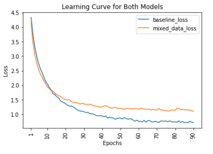
As for the model with the mixed data, it consisted of a VGG-19 network, with a “GlobalAveragePooling2D” layer, a Dropout of 0.2 probability layer, a Dense layer with 128 neurons, another Dropout of 0.5 probability layer, and a BatchNormalization layer. As with the basemodel, “Sparse Categorical Crossentropy” and the Adam Optimizer were used. About \(\frac{1}{4}\) of the VGG-19 layers were froze and 160 epochs were used to train.

With these models, we tested them with their respected testing sets. With a training accuracy of 70%, the baseline model was able to obtain an accuracy of 34%. Figure 9 displays some of the optotypes that the baseline model was able to predict correctly (with predicted likelihood for that label higher than 80%) , as well as incorrectly. A majority of the images that the baseline model was able to predict correctly were the images that didn’t have too much distortion. It was rare to find very distorted images. There was a variety of distortions found in the images that the model predicted incorrectly.

Figure 9: Optotypes that the baseline model predicted correctly (left) and incorrectly (right).

Mixed Data Model

For the mixed data model, it had a training accuracy of 65.26% and a testing accuracy of 62.88%. Figure 10 displays some of the optotypes the model predicted correctly (with predicted likelihood for that label higher than 80%) and incorrectly. From the images that the mixed model predicted correctly, there were more high-distorted images found than in the images that the baseline mode predicted correctly. There were still some medium-distorted images that the mixed model predicted incorrectly, but a majority of the images were distorted beyond recognition, as seen in the figure.

Figure 10: Optotypes that the mixed data model predicted correctly (left) and incorrectly (right).

For some of the optotypes with high amounts of distortions, we tested to see how well the mixed model was able to predict the optotypes, compared to the baseline model. The figure below (Figure 11) displays a few examples in which the mixed model was able to predict the correct label, with both high and low likelihoods of that choice, along with the baseline model’s prediction.

Figure 11: Optotype prediction comparison of the two models.

There were some optotypes that both models predicted incorrectly, which are shown in Figure 11. Most of the images that both predicted incorrectly involved a variation of “x” or “+”. The main optotypes that the models get confused with are: [“+blank”, “+circle”, “+diamond”, “+square”] and [“x-blank”, “x-circle”, “x-diamond”, “x-square”]. With high distortions, the shape in the middle of the “x” or “+” become non-recognizable, causing the model to be confused. It predicts the correct shape, but not the details of that shape. Other points of confusion included high distortions of the rotated “C” variations and variations of “O”.

Figure 12: Optotypes both model predicted incorrectly.

Data Augmentation

Data Augmentation was additionally leveraged as is a standard technique in the literature [2]. Figure 13 shows the original discrepancy between the training and testing dataset, which was extremely skewed toward the testing side.

Figure 13: Training/Testing data split before and after applying data augmentation. Training dataset gained an additional 9,000+ images.

The specific technique chosen for augmentation must be carefully selected, as traditional data augmentation techniques such as rotating, cropping, etc. would alter the integrity of the data and skew the original distortions provided, rendering the provided labels now inaccurate. The techniques chosen to bolster the training data were increasing the brightness and contrast 20%, decreasing the brightness and contrast by 20%, and then converting the image to grayscale. An array of images that were augmented compared to images that were not augmented can be seen in Figure 14.

Figure 14: Array of training items bolstered by data augmentation, and classified by multiple labels. Techniques applied include brightness adjustment, contrast adjustment, and converting to grayscale.

Data Wrangling

Real-world data, such as the dataset obtained for this project, needed to undergo intensive preprocessing to obtain several levels of labels that may be later used for analysis. For each image, the labels extracted included Acuity, Character Type (such as wingding, alpha, numeric, or symbol), the Optotype, Angle of Rotation, Level of Distortion, Image Size, and Augmentation.

While we did not have time to explore the correlations between the results and all of these labels, we did explore the relationship between the optotypes and angles.

The original dataset contained optotypes C-0, E-0, C-45, E-45, etc. One question we sought to explore was if we separated the angles from these optotypes would this increase the efficacy of the system? This decreased the optotypes from 64 to 59. We plan on creating a multi-output system where it must additionally classify the angle of rotation. The goal with this is to create a system that parallels human categorization.

Figure 15: Validation loss, comparing variations of VGG16, as well as variations in optotype classification, with and without additional data wrangling applied.

Evaluation of Results

As expected, the augmented training dataset increased the validation and training accuracy significantly. As shown in Table 1, accuracy for the network to classify low distortion, large images went up significantly—from the 60s to the low 90s. This is about as high as we could expect it to go without risking overfitting. Interestingly, though, the data augmentation/wrangling seemed to reduce the efficacy in classification of the test data. This could be for several reasons. Without the included angle in the optotypes, it is possible the network may have confused a backwards E for instance with a 3. This kind of example is demonstrated in figure 12.

Table 1: Comparison of results amongst data augmentation and wrangling techniques applied.

Conclusion

While this overall research project is still a work-in-progress, much has been gained this quarter through the opportunity to utilize in-class time, and particularly, to be able to apply concepts from this course.

Comparison to Human Results

While it was touted that one of the primary goals of the project is to compare the machine results to those of humans, those comparisons are notably missing from the report. This is because the human trials are being carried out by the Browne lab, and the app being used to conduct those trials was just released last week. To prepare for the comparison of these results, we still have some work to do, but we eagerly await the opportunity to compare the results.

Neural Networks as a Model of Human Vision

For my personal research agenda, one of the areas I’m interested in exploring are the parallels between our own human intelligence and biology and that of machines–what can we learn from each other? What gaps in machine learning are present that we can leverage biology and cognitive science to inspire our algorithms? While we have not yet had the opportunity to compare between the human results, I am further convinced from this project that neural models are an effective model of the human nervous system, and they particularly excel in problems related to computer vision.

Future Directions

One area I would like to explore in the future, which will probably be over the summer, in this project is how might an individual’s level of literacy affect the results of the acuity test? Would a literate individual, who has effectively been “trained” on significantly more alphanumeric data than an illiterate person, perform better on alphanumeric optotypes even if those two people had equally poor eyesight? I focused much of my efforts this quarter, which would have surprised me in retrospect, on data wrangling, and provided a set of custom labels to images that are alphanumeric characters that can later be used for analysis.

References

[1] Karen Simonyan and Andrew Zisserman. Very deep convolutional networks for large-scale image recognition, 2015.

[2] Sebastien C. Wong, Adam Gatt, Victor Stamatescu, and Mark D. McDonnell. Understanding data augmentation for classification: when to warp?, 2016.13

Appendix

Code

The code can be viewed on GitHub here: GitHub Visual Acuity.

I wrote quite a bit of code for this project, so I’ll summarize here the module structure that delineates what to find in the .zip file. All of the code included was written by me, and I did of course leverage Deep Learning libraries like tensorflow, keras, etc.

• config: contains the YAML files with the training parameters
• data: contains a helper class Dataset that I wrote which loads in the pickled processed image data
• model: contains code I wrote for the VGG16 transfer model
• preprocessing: this is all of the code used to preprocess and categorize all of the image data from the original dataset
• Teller: sub-module of preprocessing, special processing that was applied to Teller acuities.
• util: contains a utility method to connect my runs to Weights and Biases to produce visualizations.
• main.py: entry point to the program

Data Visualization

Weights and Biases was used to produce some of the graphs and store data from the runs. The project can be viewed here: WandB Visual Acuity.

Link to Dataset

The original dataset, aggregated by the Browne Lab, can be viewed and downloaded here: DropBox.